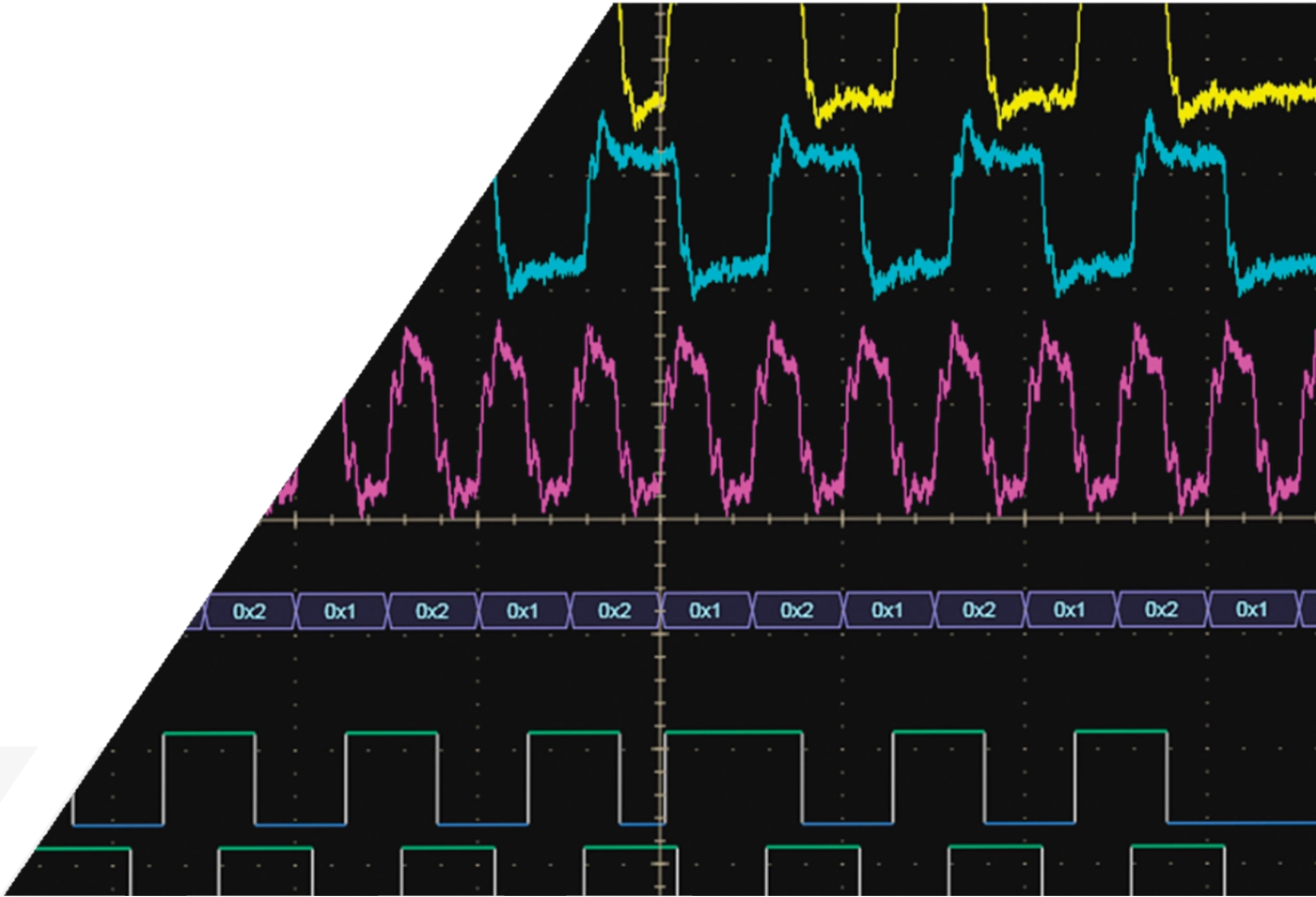
Introduction

Nature moves in the form of a sine wave, be it an ocean wave, earthquake, sonic boom, explosion, sound through air, or the natural frequency of a body in motion. Energy, vibrating particles and other invisible forces pervade our physical universe. Even light – part particle, part wave – has a fundamental frequency, which can be observed as color.

Sensors can convert these forces into electrical signals that you can observe and study with an oscilloscope. Oscilloscopes enable scientists, engineers, technicians, educators and others to “see” events that change over time.

Oscilloscopes are indispensable tools for anyone designing, manufacturing or repairing electronic equipment. In today’s fast-paced world, engineers need the best tools available to solve their measurement challenges quickly and accurately. As the eyes of the engineer, oscilloscopes are the key to meeting today’s demanding measurement challenges.

The usefulness of an oscilloscope is not limited to the world of electronics. With the proper sensor, an oscilloscope can measure all kinds of phenomena. A sensor is a device that creates an electrical signal in response to physical stimuli, such as sound, mechanical stress, pressure, light, or heat. A microphone is a sensor that converts sound into an electrical signal. Figure 1 shows an example of scientific data that can be gathered by an oscilloscope.

Oscilloscopes are used by everyone from physicists to repair technicians. An automotive engineer uses an oscilloscope to correlate analog data from sensors with serial data from the engine control unit. A medical researcher uses an oscillscope to measure brain waves. The possibilities are endless.

The concepts presented in this primer will provide you with a good starting point in understanding oscilloscope basics and operation.

Figure 1. An example of scientific data gathered by an oscilloscope.

The glossary in the back of this primer will give you definitions of unfamiliar terms. The vocabulary and multiple-choice written exercises on oscilloscope theory and controls make this primer a useful classroom aid. No mathematical or electronics knowledge is necessary.

After reading this primer, you will be able to:

• Describe how oscilloscopes work
• Describe the differences between various oscilloscopes Describe electrical waveform types
• Understand basic oscilloscope controls
• Take simple measurements

The manual provided with your oscilloscope will give you more specific information about how to use the oscilloscope in your work. Some oscilloscope manufacturers also provide a multitude of application notes to help you optimize the oscilloscope for your application-specific measurements.

Signal Integrity

The Significance of Signal Integrity

The key to any good oscilloscope system is its ability to accurately reconstruct a waveform – referred to as signal integrity. An oscilloscope is analogous to a camera that captures signal images that we can then observe and interpret. Two key issues lie at the heart of signal integrity.

• When you take a picture, is it an accurate picture of what actually happened?
• Is the picture clear or fuzzy?
• How many of those accurate pictures can you take per second?

Taken together, the different systems and performance capabilities of an oscilloscope contribute to its ability to deliver the highest signal integrity possible. Probes also affect the signal integrity of a measurement system.

Signal integrity impacts many electronic design disciplines. But until a few years ago, it wasn’t much of a problem for digital designers. They could rely on their logic designs to act like the Boolean circuits they were. Noisy, indeterminate signals were something that occurred in high-speed designs – something for RF designers to worry about. Digital systems switched slowly and signals stabilized predictably.

Processor clock rates have since multiplied by orders of magnitude. Computer applications such as 3D graphics, video and server I/O demand vast bandwidth. Much of today’s telecommunications equipment is digitally based, and similarly requires massive bandwidth. So too does digital high-definition TV. The current crop of microprocessor devices handles data at rates up to 2, 3 and even 5 GS/s (gigasamples per second), while some DDR3 memory devices use clocks in excess of
2 GHz as well as data signals with 35 ps rise times.
Importantly, speed increases have trickled down to the common IC devices used in automobiles, consumer electronics, and machine controllers, to name just a few applications.

A processor running at a 20 MHz clock rate may well have signals with rise times similar to those of an 800 MHz processor. Designers have crossed a performance threshold that means, in effect, almost every design is a high-speed design.

Without some precautionary measures, high-speed problems can creep into otherwise conventional digital designs. If a circuit is experiencing intermittent failures, or if it encounters errors at voltage and temperature extremes, chances are there are some hidden signal integrity problems. These can affect time-to-market, product reliability, EMI compliance, and more. These high-speed problems can also impact the integrity of a serial data stream in a system, requiring some method of correlating specific patterns in the data with the observed characteristics of high-speed waveforms.

Why is Signal Integrity a Problem?

Let’s look at some of the specific causes of signal degradation in today’s digital designs. Why are these problems so much more prevalent today than in years past?

The answer is speed. In the “slow old days,” maintaining acceptable digital signal integrity meant paying attention
to details like clock distribution, signal path design, noise margins, loading effects, transmission line effects, bus termination, decoupling and power distribution. All of these rules still apply, but…

Bus cycle times are up to a thousand times faster than they were 20 years ago! Transactions that once took microseconds are now measured in nanoseconds. To achieve this improvement, edge speeds too have accelerated: they are up to 100 times faster than those of two decades ago.

This is all well and good; however, certain physical realities have kept circuit board technology from keeping up the pace. The propagation time of inter-chip buses has remained almost unchanged over the decades. Geometries have shrunk, certainly, but there is still a need to provide circuit board real estate for IC devices, connectors, passive components, and of course, the bus traces themselves. This real estate adds up to distance, and distance means time – the enemy of speed.

It’s important to remember that the edge speed – rise time – of a digital signal can carry much higher frequency components than its repetition rate might imply. For this reason, some designers deliberately seek IC devices with relatively “slow” rise times.
The lumped circuit model has always been the basis of most calculations used to predict signal behavior in a circuit. But when edge speeds are more than four to six times faster than the signal path delay, the simple lumped model no longer applies.

Circuit board traces just six inches long become transmission lines when driven with signals exhibiting edge rates below four to six nanoseconds, irrespective of the cycle rate. In effect, new signal paths are created. These intangible connections aren’t on the schematics, but nevertheless provide a means for signals to influence one another in unpredictable ways.

Sometimes even the errors introduced by the probe/instrument combination can provide a significant contribution to the signal being measured. However, by applying the “square root of the sum of the squares” formula to the measured value, it is possible to determine whether the device under test is approaching a rise/fall time failure. In addition, recent oscilloscope tools use special filtering techniques to de-embed the measurement system’s effects on the signal, displaying edge times and other signal characteristics.

At the same time, the intended signal paths don’t work the way they are supposed to. Ground planes and power planes, like the signal traces described above, become inductive and act like transmission lines; power supply decoupling is far less effective. EMI goes up as faster edge speeds produce shorter wavelengths relative to the bus length. Crosstalk increases.
In addition, fast edge speeds require generally higher currents to produce them. Higher currents tend to cause ground bounce, especially on wide buses in which many signals switch at once. Moreover, higher current increases the amount of radiated magnetic energy and with it, crosstalk.

Viewing the Analog Origins of Digital Signals

What do all these characteristics have in common? They are classic analog phenomena. To solve signal integrity problems, digital designers need to step into the analog domain. And to take that step, they need tools that can show them how digital and analog signals interact.

Digital errors often have their roots in analog signal integrity problems. To track down the cause of the digital fault,
it’s often necessary to turn to an oscilloscope, which can display waveform details, edges and noise; can detect and display transients; and can help you precisely measure timing relationships such as setup and hold times. Modern oscilloscopes can help to simplify the troubleshooting process by triggering on specific patterns in parallel or serial data streams and displaying the analog signal that corresponds in time with a specified event.

Understanding each of the systems within your oscilloscope and how to apply them will contribute to the effective application of the oscilloscope to tackle your specific measurement challenge.

Figure 2. X, Y, and Z components of a displayed waveform.

The Oscilloscope

What is an oscilloscope and how does it work? This section answers these fundamental questions.

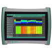
The oscilloscope is basically a graph-displaying device – it draws a graph of an electrical signal. In most applications, the graph shows how signals change over time: the vertical (Y) axis represents voltage and the horizontal (X) axis represents time. The intensity or brightness of the display is sometimes called the Z axis, as shown in Figure 2. In DPO oscilloscopes, the Z axis can be represented by color grading of the display, as seen in Figure 3.

This simple graph can tell you many things about a signal, such as:

• The time and voltage values of a signal
• The frequency of an oscillating signal
• The “moving parts” of a circuit represented by the signal
• The frequency with which a particular portion of the signal is occurring relative to other portions
• Whether or not a malfunctioning component is distorting the signal
• How much of a signal is direct current (DC) or alternating current (AC)
• How much of the signal is noise and whether the noise is changing with time

Figure 3. Two offset clock patterns with Z axis intensity grading.

Understanding Waveforms and Waveform Measurements

The generic term for a pattern that repeats over time is a wave – sound waves, brain waves, ocean waves, and voltage waves are all repetitive patterns. An oscilloscope measures voltage waves. Remember as mentioned earlier, that physical phenomena such as vibrations or temperature or electrical phenomena such as current or power can be converted to a voltage by a sensor. One cycle of a wave is the portion of the wave that repeats. A waveform is a graphic representation of a wave. A voltage waveform shows time on the horizontal axis and voltage on the vertical axis.

Figure 4. Common waveforms.

Waveform shapes reveal a great deal about a signal. Any time you see a change in the height of the waveform, you know the voltage has changed. Any time there is a flat horizontal line, you know that there is no change for that length of time. Straight, diagonal lines mean a linear change – rise or fall of voltage at a steady rate. Sharp angles on a waveform indicate sudden change. Figure 4 shows common waveforms and Figure 5 displays sources of common waveforms.

Figure 5. Sources of common waveforms.

Types of Waves

You can classify most waves into these types:

• Sine waves
• Square and rectangular waves
• Sawtooth and triangle waves
• Step and pulse shapes
• Periodic and non-periodic signals
• Synchronous and asynchronous signals
• Complex waves

Sine Waves

The sine wave is the fundamental wave shape for several reasons. It has harmonious mathematical properties – it is the same sine shape you may have studied in trigonometry class. The voltage in your wall outlet varies as a sine wave. Test signals produced by the oscillator circuit of a signal generator are often sine waves. Most AC power sources produce sine waves. (AC signifies alternating current, although the voltage alternates too. DC stands for direct current, which means a steady current and voltage, such as a battery produces.)
The damped sine wave is a special case you may see in a circuit that oscillates, but winds down over time.

Square and Rectangular Waves

The square wave is another common wave shape. Basically, a square wave is a voltage that turns on and off (or goes high and low) at regular intervals. It is a standard wave for testing amplifiers – good amplifiers increase the amplitude of a square wave with minimum distortion. Television, radio and computer circuitry often use square waves for timing signals.

The rectangular wave is like the square wave except that
the high and low time intervals are not of equal length. It is particularly important when analyzing digital circuitry.

Sawtooth and Triangle Waves

Sawtooth and triangle waves result from circuits designed
to control voltages linearly, such as the horizontal sweep of an analog oscilloscope or the raster scan of a television. The transitions between voltage levels of these waves change at a constant rate. These transitions are called ramps.

Step and Pulse Shapes

Signals such as steps and pulses that occur rarely, or nonperiodically, are called single-shot or transient signals.
A step indicates a sudden change in voltage, similar to the voltage change you would see if you turned on a power switch.

A pulse indicates sudden changes in voltage, similar to
the voltage changes you would see if you turned a power switch on and then off again. A pulse might represent one bit of information traveling through a computer circuit or it might be a glitch, or defect, in a circuit. A collection of pulses traveling together creates a pulse train. Digital components in a computer communicate with each other using pulses. These pulses may be in the form of serial data stream or multiple signal lines may be used to represent a value in a parallel data bus. Pulses are also common in x-ray, radar, and communications equipment.

Periodic and Non-periodic Signals

Repetitive signals are referred to as periodic signals, while signals that constantly change are known as non-periodic signals. A still picture is analogous to a periodic signal, while a moving picture can be equated to a non-periodic signal.

Synchronous and Asynchronous Signals

When a timing relationship exists between two signals, those signals are referred to as synchronous. Clock, data and address signals inside a computer are an example of synchronous signals.

Asynchronous is a term used to describe those signals between which no timing relationship exists. Because no time correlation exists between the act of touching a key on a computer keyboard and the clock inside the computer, these are considered asynchronous.

Figure 6. An NTSC composite video signal is an example of a complex wave.

Complex Waves

Some waveforms combine the characteristics of sines, squares, steps, and pulses to produce complex waveshapes. The signal information may be embedded in the form of amplitude, phase, and/or frequency variations. For example, although the signal in Figure 6 is an ordinary composite video signal, it is composed of many cycles of higher-frequency waveforms embedded in a lower-frequency envelope.

In this example, it is usually most important to understand the relative levels and timing relationships of the steps. To view this signal, you need an oscilloscope that captures the low-frequency envelope and blends in the higher-frequency waves in an intensity-graded fashion so that you can see their overall combination as an image that can be visually interpreted. Digital phosphor oscilloscopes are most suited to viewing complex waves, such as video signals, illustrated in Figure 6. Their displays provide the necessary frequency-of-occurrence information, or intensity grading, that is essential to understanding what the waveform is really doing.

Figure 7. 622 Mb/s serial data eye pattern.

Some oscilloscopes allow for displaying certain types
of complex waveforms in special ways. For example, telecommunications data may be displayed as an eye pattern or a constellation diagram.

Telecommunications digital data signals can be displayed on an oscilloscope as a special type of waveform referred to as an eye pattern. The name comes from the similarity of the waveform to a series of eyes, as seen in Figure 7. Eye patterns are produced when digital data from a receiver is sampled and applied to the vertical input, while the data rate is used to trigger the horizontal sweep. The eye pattern displays one bit or unit interval of data with all possible edge transitions and states superimposed in one comprehensive view.

A constellation diagram is a representation of a signal modulated by a digital modulation scheme such as quadrature amplitude modulation or phase-shift keying.

Figure 8. Frequency and period of a sine wave.

Waveform Measurements

Many terms are used to describe the types of measurements that you make with your oscilloscope. This section describes some of the most common measurements and terms.

Frequency and Period

If a signal repeats, it has a frequency. The frequency is measured in Hertz (Hz) and equals the number of times the signal repeats itself in one second, referred to as cycles per second. A repetitive signal also has a period, which is the amount of time it takes the signal to complete one cycle. Period and frequency are reciprocals of each other, so that 1/period equals the frequency and 1/frequency equals the period. For example, the sine wave in Figure 8 has a frequency of 3 Hz and a period of 1/3 second.

Voltage

Voltage is the amount of electric potential, or signal strength, between two points in a circuit. Usually, one of these points is ground, or zero volts, but not always. You may want to measure the voltage from the maximum peak to the minimum peak of a waveform, referred to as the peak-to-peak voltage.

Amplitude

Amplitude refers to the amount of voltage between two points in a circuit. Amplitude commonly refers to the maximum voltage of a signal measured from ground, or zero volts. The waveform shown in Figure 9 has an amplitude of 1 V and a peak-to-peak voltage of 2 V.

Figure 9. Amplitude and degrees of a sine wave.

Figure 10. Phase shift.

Phase

Phase is best explained by looking at a sine wave. The voltage level of sine waves is based on circular motion. Given that a circle has 360°, one cycle of a sine wave has 360°, as shown in Figure 9. Using degrees, you can refer to the phase angle of a sine wave when you want to describe how much of the period has elapsed.

Phase shift describes the difference in timing between two otherwise similar signals. The waveform in Figure 10 labeled “current” is said to be 90° out of phase with the waveform labeled “voltage,” since the waves reach similar points in their cycles exactly 1/4 of a cycle apart (360°/4 = 90°). Phase shifts are common in electronics.

Waveform Measurements with Digital Oscilloscopes

Modern digital oscilloscopes have functions that make waveform measurements easier. They have front-panel buttons and/or screen-based menus from which you
can select fully automated measurements. These include amplitude, period, rise/fall time, and many more. Many digital instruments also provide mean and RMS calculations, duty cycle, and other math operations. Automated measurements appear as on-screen alphanumeric readouts. Typically these readings are more accurate than is possible to obtain with direct graticule interpretation.

Examples of fully automated waveform measurements:

• Period
• Frequency
• Width +
• Width -
• Rise time
• Fall time
• Amplitude
• Duty Cycle +
• Duty Cycle -
• Delay
• Phase
• Burst width
• Peak-to-peak
• High
• Low
• Minimum
• Maximum
• Overshoot +
• Overshoot -
• RMS
• Cycle RMS
• Jitter

The Types of Oscilloscopes

Electronic equipment can be classified into two categories: analog and digital. Analog equipment works with continuously variable voltages, while digital equipment works with discrete binary numbers that represent voltage samples.
A conventional phonograph is an analog device, while a compact disc player is a digital device.

Oscilloscopes can be classified similarly – as analog and digital types. In contrast to an analog oscilloscope, a digital oscilloscope uses an analog-to-digital converter (ADC) to convert the measured voltage into digital information. It acquires the waveform as a series of samples, and stores these samples until it accumulates enough samples to describe a waveform. The digital oscilloscope then re-assembles the waveform for display on the screen, as seen in Figure 11.

Digital oscilloscopes can be classified into digital storage oscilloscopes (DSOs), digital phosphor oscilloscopes (DPOs), mixed signal oscilloscopes (MSOs), and digital sampling oscilloscopes.

The digital approach means that the oscilloscope can display any frequency within its range with stability, brightness, and clarity. For repetitive signals, the bandwidth of the digital oscilloscope is a function of the analog bandwidth of the

front-end components of the oscilloscope, commonly referred to as the –3 dB point. For single-shot and transient events, such as pulses and steps, the bandwidth can be limited by the oscilloscope’s sample rate. Please refer to the Sample Rate section under Performance Terms and Considerations for a more detailed discussion.

Digital Storage Oscilloscopes

A conventional digital oscilloscope is known as a digital storage oscilloscope (DSO). Its display typically relies on a raster-type screen rather than the luminous phosphor found in an older analog oscilloscope.

Digital storage oscilloscopes (DSOs) allow you to capture and view events that may happen only once – known as transients. Because the waveform information exists in digital form as a series of stored binary values, it can be analyzed, archived, printed, and otherwise processed, within the oscilloscope itself or by an external computer. The waveform need not be continuous; it can be displayed even when the signal disappears. Unlike analog oscilloscopes, digital storage oscilloscopes provide permanent signal storage and extensive waveform processing. However, DSOs typically have no real-time intensity grading; therefore, they cannot express varying levels of intensity in the live signal.

Some of the subsystems that comprise DSOs are similar
to those in analog oscilloscopes. However, DSOs contain additional data-processing subsystems that are used to collect and display data for the entire waveform. A DSO employs a serial-processing architecture to capture and display a signal on its screen, as shown in Figure 12. A description of this serial-processing architecture follows.

Serial-processing Architecture

Like an analog oscilloscope, a DSO’s first (input) stage is
a vertical amplifier. Vertical controls allow you to adjust the amplitude and position range at this stage. Next, the analogto- digital converter (ADC) in the horizontal system samples the signal at discrete points in time and converts the signal’s voltage at these points into digital values called sample points. This process is referred to as digitizing a signal.

The horizontal system’s sample clock determines how often the ADC takes a sample. This rate is referred to as the sample rate and is expressed in samples per second (S/s). The sample points from the ADC are stored in acquisition memory as waveform points. Several sample points may comprise one waveform point. Together, the waveform points comprise one waveform record. The number of waveform points used to create a waveform record is called the record length. The trigger system determines the start and stop points of the record.

The DSO’s signal path includes a microprocessor through which the measured signal passes on its way to the display. This microprocessor processes the signal, coordinates display activities, manages the front panel controls, and more. The signal then passes through the display memory and is displayed on the oscilloscope screen.

Figure 13. The digital storage oscilloscope delivers high-speed, single-shot acquisition across multiple channels, increasing the likelihood of capturing elusive glitchesand transient events.

Depending on the capabilities of your oscilloscope, additional processing of the sample points may take place, which enhances the display. Pre-trigger may also be available, enabling you to see events before the trigger point. Most
of today’s digital oscilloscopes also provide a selection
of automatic parametric measurements, simplifying the measurement process.

As shown in Figure 13, a DSO provides high performance in a single-shot, multi-channel instrument. DSOs are ideal for low-repetition-rate or single-shot, high-speed, multichannel design applications. In the real world of digital design, an engineer usually examines four or more signals simultaneously, making the DSO a critical companion.

Digital Phosphor Oscilloscopes

The digital phosphor oscilloscope (DPO) offers a new approach to oscilloscope architecture. This architecture enables a DPO to deliver unique acquisition and display capabilities to accurately reconstruct a signal.

While a DSO uses a serial-processing architecture to capture, display and analyze signals, a DPO employs a parallel-processing architecture to perform these functions, as shown in Figure 14. The DPO architecture dedicates unique ASIC hardware to acquire waveform images, delivering high waveform capture rates that result in a higher level of signal visualization. This performance increases the probability of witnessing transient events that occur in digital systems, such as runt pulses, glitches and transition errors, and enables additional analysis capability. A description of this parallel-processing architecture follows.

Parallel-processing Architecture

A DPO’s first (input) stage is similar to that of an analog oscilloscope – a vertical amplifier – and its second stage
is similar to that of a DSO – an ADC. But, the DPO differs significantly from its predecessors following the analog-todigital conversion.

For any oscilloscope – analog, DSO or DPO – there is always a holdoff time during which the instrument processes the most recently acquired data, resets the system, and waits for the next trigger event. During this time, the oscilloscope is blind to all signal activity. The probability of seeing an infrequent or low-repetition event decreases as the holdoff time increases.

It should be noted that it is impossible to determine the
probability of capture by simply looking at the display update rate. If you rely solely on the update rate, it is easy to make the mistake of believing that the oscilloscope is capturing all pertinent information about the waveform when, in fact, it is not.

The digital storage oscilloscope processes captured waveforms serially. The speed of its microprocessor is a bottleneck in this process because it limits the waveform capture rate. The DPO rasterizes the digitized waveform data into a digital phosphor database. Every 1/30th of a second – about as fast as the human eye can perceive it – a snapshot of the signal image that is stored in the database is pipelined directly to the display system. This direct rasterization of waveform data, and direct copy to display memory from the database, removes the data-processing bottleneck inherent in other architectures. The result is an enhanced “real-time” and lively display update. Signal details, intermittent events, and dynamic characteristics of the signal are captured in realtime. The DPO’s microprocessor works in parallel with this integrated acquisition system for display management, measurement automation and instrument control, so that it does not affect the oscilloscope’s acquisition speed.

A DPO faithfully emulates the best display attributes of an analog oscilloscope, displaying the signal in three dimensions: time, amplitude and the distribution of amplitude over time, all in real-time.

Figure 15. Some DPOs can acquire millions of waveform in just seconds, significantly increasing the probability of capturing intermittent and elusive events and revealing dynamic signal behavior.

Unlike an analog oscilloscope’s reliance on chemical phosphor, a DPO uses a purely electronic digital phosphor that’s actually a continuously updated database. This database has a separate “cell” of information for every single pixel in the oscilloscope’s display. Each time a waveform is captured – in other words, every time the oscilloscope triggers – it is mapped into the digital phosphor database’s cells. Each cell that represents a screen location and is touched by the waveform is reinforced with intensity information, while other cells are not. Thus, intensity information builds up in cells where the waveform passes most often.

When the digital phosphor database is fed to the oscilloscope’s display, the display reveals intensified waveform areas, in proportion to the signal’s frequency of occurrence at each point – much like the intensity grading characteristics of an analog oscilloscope. The DPO also allows the display of the varying frequency-of-occurrence information on the display as contrasting colors, unlike an analog oscilloscope. With a DPO, it is easy to see the difference between a waveform that occurs on almost every trigger and one that occurs, say, every 100th trigger.

Digital phosphor oscilloscopes (DPOs) break down the barrier between analog and digital oscilloscope technologies. They are equally suitable for viewing high and low frequencies, repetitive waveforms, transients, and signal variations in realtime. Only a DPO provides the Z (intensity) axis in real-time that is missing from conventional DSOs.

A DPO is ideal for those who need the best general-purpose design and troubleshooting tool for a wide range of applications, as seen in Figure 15. A DPO is exemplary for advanced analysis, communication mask testing, digital debug of intermittent signals, repetitive digital design and timing applications.

Figure 16. Time-correlated display of a Zigbee radio's microprocessor SPI (MOSI) and (MISO) control lines, with measurements of drain current and voltage to the radio IC and the spectrum during turn-on.

Mixed Domain Oscilloscopes

A mixed domain oscilloscope (MDO) combines an RF spectrum analyzer with a MSO or DPO to enable correlated views of signals from the digital, analog, to RF domains. For example, the MDO allows you to view time-correlated displays of protocol, state logic, analog, and RF signals within an embedded design. This dramatically reduces both the time to insight and the measurement uncertainty between cross domain events.

Understanding the time delay between a microprocessor command and a RF event within an embedded RF design simplifies test setups and brings complex measurements to the bench. For embedded radios, such as the Zigbee design shown in Figure 16, you can trigger on the turn-on
of the RF event and view the command line latency of the microprocessor controller decoded SPI control lines, the drain current and voltage during turn-on, and any spectral events that result. In one display, you now have a time-correlated view of all the domains of the radio: protocol (digital), analog, and RF.

Figure 17. The MSO provides 16 integrated digital channels, enabling the ability to view and analyze time-correlated analog and digital signals.

Mixed Signal Oscilloscopes

The mixed signal oscilloscope (MSO) combines the performance of a DPO with the basic functionality of a
16-channel logic analyzer, including parallel/serial bus protocol decoding and triggering. The MSO's digital channels view a digital signal as either a logic high or logic low, just like a digital circuit views the signal. This means as long as ringing, overshoot and ground bounce do not cause logic transitions, these analog characteristics are not of concern to the MSO. Just like a logic analyzer, a MSO uses a threshold voltage to determine if the signal is logic high or logic low.

The MSO is the tool of choice for quickly debugging digital circuits using its powerful digital triggering, high resolution acquisition capability, and analysis tools. The root cause of many digital problems is quicker to pinpoint by analyzing both the analog and digital representations of the signal, as shown in Figure 17, making a MSO ideal for verifying and debugging digital circuits.

Digital Sampling Oscilloscopes

In contrast to the digital storage and digital phosphor oscilloscope architectures, the architecture of the digital sampling oscilloscope reverses the position of the attenuator/ amplifier and the sampling bridge, as shown in Figure 18. The input signal is sampled before any attenuation or amplification is performed. A low bandwidth amplifier can then be utilized after the sampling bridge because the signal has already been converted to a lower frequency by the sampling gate, resulting in a much higher bandwidth instrument.

The tradeoff for this high bandwidth, however, is that the sampling oscilloscope’s dynamic range is limited. Since there is no attenuator/amplifier in front of the sampling gate, there is no facility to scale the input. The sampling bridge must be able to handle the full dynamic range of the input at all times. Therefore, the dynamic range of most sampling oscilloscopes is limited to about 1 V peak-to-peak. Digital storage and digital phosphor oscilloscopes, on the other hand, can handle 50 to 100 volts.

In addition, protection diodes cannot be placed in front of the sampling bridge as this would limit the bandwidth. This reduces the safe input voltage for a sampling oscilloscope
to about 3 V, as compared to 500 V available on other oscilloscopes.

Figure 19. Time domain reflectometry (TDR) display from a digital sampling oscilloscope.

When measuring high-frequency signals, the DSO or DPO may not be able to collect enough samples in one sweep.
A digital sampling oscilloscope is an ideal tool for accurately capturing signals whose frequency components are much higher than the oscilloscope’s sample rate, as seen in
Figure 19. This oscilloscope is capable of measuring
signals of up to an order of magnitude faster than any other oscilloscope. It can achieve bandwidth and high-speed timing ten times higher than other oscilloscopes for repetitive signals. Sequential equivalent-time sampling oscilloscopes are available with bandwidths to 80 GHz.

The Systems and Controls of an
Oscilloscope

This section briefly describes the basic systems and controls found on analog and digital oscilloscopes. Some controls differ between analog and digital oscilloscopes; your oscilloscope probably has additional controls not discussed here.

A basic oscilloscope consists of four different systems – the vertical system, horizontal system, trigger system, and display system. Understand-ing each of these systems will enable you to effectively apply the oscilloscope to tackle your specific measurement challenges. Recall that each system contributes to the oscilloscope’s ability to accurately reconstruct a signal.

The front panel of an oscilloscope is divided into three main sections labeled vertical, horizontal, and trigger. Your oscilloscope may have other sections, depending on the model and type. See if you can locate these front-panel sections in Figure 20, and on your oscilloscope, as you read through this section.

When using an oscilloscope, you need to adjust three basic settings to accommodate an incoming signal:

• Vertical: The attenuation or amplification of the signal. Use the volts/div control to adjust the amplitude of the signal to the desired measurement range.
• Horizontal: The time base. Use the sec/div control to set the amount of time per division represented horizontally across the screen.
• Trigger: The triggering of the oscilloscope. Use the trigger level to stabilize a repeating signal, or to trigger on a single event.

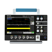
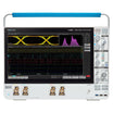
Figure 20. Front-panel control section of an oscilloscope.

Common vertical controls include:

• Termination
  - 1M ohm
  - 50 ohm
• Coupling
  - DC
  - AC
  - GND
• Bandwidth
  - Limit
  - Enhancement
• Position
• Offset
• Invert – On/Off
• Scale
  - Fixed steps
  - Variable

Vertical System and Controls

Vertical controls can be used to position and scale the waveform vertically, set the input coupling, and adjust other signal conditioning.

Position and Volts per Division

The vertical position control allows you to move the waveform up and down exactly where you want it on the screen.

The volts-per-division setting (usually written as volts/div) is a scaling factor that varies the size of the waveform on the screen. If the volts/div setting is 5 volts, then each of the eight vertical divisions represents 5 volts and the entire screen can display 40 volts from bottom to top, assuming a graticule with eight major divisions. If the setting is 0.5 volts/div, the screen can display 4 volts from bottom to top, and so on. The maximum voltage you can display on the screen is the volts/div setting multiplied by the number of vertical divisions. Note that the probe you use, 1X or 10X, also influences the scale factor. You must divide the volts/div scale by the attenuation factor of the probe if the oscilloscope does not do it for you.

Often the volts/div scale has either a variable gain or a fine gain control for scaling a displayed signal to a certain number of divisions. Use this control to assist in taking rise time measurements.

Input Coupling

Coupling refers to the method used to connect an electrical signal from one circuit to another. In this case, the input coupling is the connection from your test circuit to the oscilloscope. The coupling can be set to DC, AC, or ground. DC coupling shows all of an input signal. AC coupling blocks the DC component of a signal so that you see the waveform centered around zero volts. Figure 21 illustrates this difference. The AC coupling setting is useful when the entire signal (alternating current + direct current) is too large for the volts/div setting.

The ground setting disconnects the input signal from the vertical system, which lets you see where zero volts is located on the screen. With grounded input coupling and auto trigger mode, you see a horizontal line on the screen that represents zero volts. Switching from DC to ground and back again is a handy way of measuring signal voltage levels with respect to ground.

Bandwidth Limit

Most oscilloscopes have a circuit that limits the bandwidth of the oscilloscope. By limiting the bandwidth, you reduce the noise that sometimes appears on the displayed waveform, resulting in a cleaner signal display. Note that, while eliminating noise, the bandwidth limit can also reduce or eliminate high-frequency signal content.

Bandwidth Enhancement

Some oscilloscopes may provide a DSP arbitrary equalization filter which can be used to improve the oscilloscope channel response. This filter extends the bandwidth, flattens the oscilloscope channel frequency response, improves phase linearity, and provides a better match between channels. It also decreases rise time and improves the time domain step response.

Horizontal System and Controls

An oscilloscope’s horizontal system is most closely associated with its acquisition of an input signal – sample rate and record length are among the considerations here. Horizontal controls are used to position and scale the waveform horizontally.

Acquisition Controls

Digital oscilloscopes have settings that let you control how the acquisition system processes a signal. Look over the acquisition options on your digital oscilloscope while you read this description. Figure 22 shows you an example of an acquisition menu.

Acquisition Modes

Acquisition modes control how waveform points are produced from sample points. Sample points are the digital values derived directly from the analog-to-digital converter (ADC). The sample interval refers to the time between these sample points. Waveform points are the digital values that are stored in memory and displayed to construct the waveform. The time value difference between waveform points is referred to as the waveform interval.

Common horizontal controls include:

• Time Base
• XY
• Scale
• Trace Separation
• Record Length
• Resolution
• Sample Rate
• Trigger Position
• Zoom/Pan
• Search

Figure 22. Example of an acquisition menu.

The sample interval and the waveform interval may, or may not, be the same. This fact leads to the existence of several different acquisition modes in which one waveform point is comprised of several sequentially acquired sample points.
Additionally, waveform points can be created from a composite of sample points taken from multiple acquisitions, which provides another set of acquisition modes. A description of the most commonly used acquisition modes follows.